Technical Approach
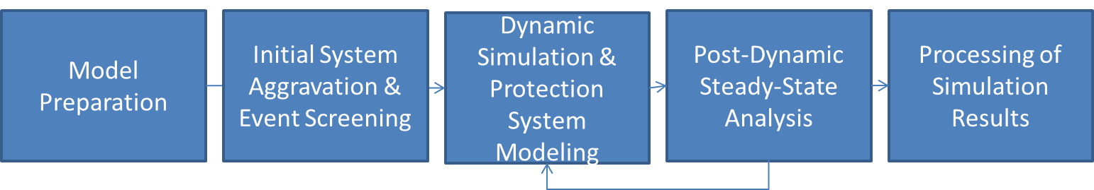
The DCAT approach consists of four main modules: model preparation, initial system aggravation and event screening, dynamic simulation and protection system modeling, and post-contingency steady-state analysis. A fifth module is used to process simulation results and log the sequence of cascading events. A flow chart of the DCAT approach modules is shown in Figure 1.
Model Preparation
The user can provide multiple base planning cases corresponding, for example, to different seasons, different levels of wind and solar penetration, different load levels, and variants of possible system reinforcements among other things, which reflect a variety of possible initial system conditions. The base planning cases include both power flow and dynamic system models.
Protection system models are added to the base cases. Selected generic relay models in Siemens PSS®E PSLF have been used in dynamic simulations as follows.
- Undervoltage, overvoltage, underfrequency, and overfrequency relays have been modeled for each generating unit. The settings of generating units’ protection relays are based on the new NERC Standard PRC-024-1, “Generator Frequency and Voltage Protective Relay Settings.
- Two types of transmission system protection were modeled:
- distance-relay protection (used in dynamic simulation). The suggested relay settings and associated operation of zones of protection are based on best practices.
- overcurrent protection (used in post-dynamic steady-state simulation). The relay settings are based on NERC Standard PRC-023-3, “Transmission Relay Loadability.”
- Two types of load shedding schemes were modeled:
- underfrequency (frequency-responsive non-firm load shedding)
- underfrequency and undervoltage firm load shedding.
- Load shedding relay settings were provided by the grid operator of the full interconnection used for simulations.
Initial System Aggravation and Event Screening
At this stage, in the general methodology, we will simulate various system states (load levels, dispatches, etc.) and light contingencies, such as N−1 contingencies. We will use power flow simulations at this stage. To select the initiating events that trigger cascading outages, a steady-state-based contingency/cascading simulation can be applied.
Dynamic Simulation
The dynamic simulation process is internally integrated with the protection system model. At each simulation step, system parameters are checked against dynamics-based protection models. Both successful and unsuccessful (due to a failure) operation of protection are simulated. For the unsuccessful outcome, new dynamic processes (cages) are started. The dynamic simulation runs until a stable point is reached, or it can be stopped if instability is detected. The instability criteria are user defined. For instance, they can include transient voltage and frequency dips, unlimited increase of phase angle differences, etc.
Dynamic simulation is a computationally intensive task. An adaptive simulation time module has been implemented to run the dynamic simulation long enough to capture the dynamic response of the system. The appropriate time can be determined by having stability checks at intermediary times that could stop the dynamic simulation. The simulation is initially run for 30 seconds; after that it runs in increments of 5 seconds.
Post-Dynamic Steady-State Analysis
The objective of post-dynamic steady-state analysis is to model special protection systems (SPS)/remedial action schemes (RAS) response, other automatic controls, and operator manual corrective actions. If these corrective actions fail to eliminate transmission lines and/or transformers overloading, slower overcurrent protection tripping actions are simulated.
The automatic control actions of transformer tap changes, switching of shunt reactors and capacitor banks, phase shifter, static compensators (STATCOM), and static VAr compensators (SVC) are used to eliminate voltage violations. The DCAT implements these actions using the PSS/E AC corrective actions function, which is part of the Multi-Level AC Contingency Computation (MACCC) application.
Operator manual actions to eliminate line overloading through generation redispatch and load shedding are modeled in the DCAT using the PSS/E AC corrective actions function.
If there are still overloaded lines after all possible corrective actions have been taken, the DCAT will select the line with the highest overloading percentage to be tripped. This process is performed through dynamic simulation as if this tripping is a new initiating event imposed on the current system topology, including all the tripping that occurred in previous cascading steps.
Simulation Results
- Demonstration of the Role of a Non-Firm Frequency-Responsive Load Shedding Scheme in Maintaining Grid Integrity after an Extreme Event
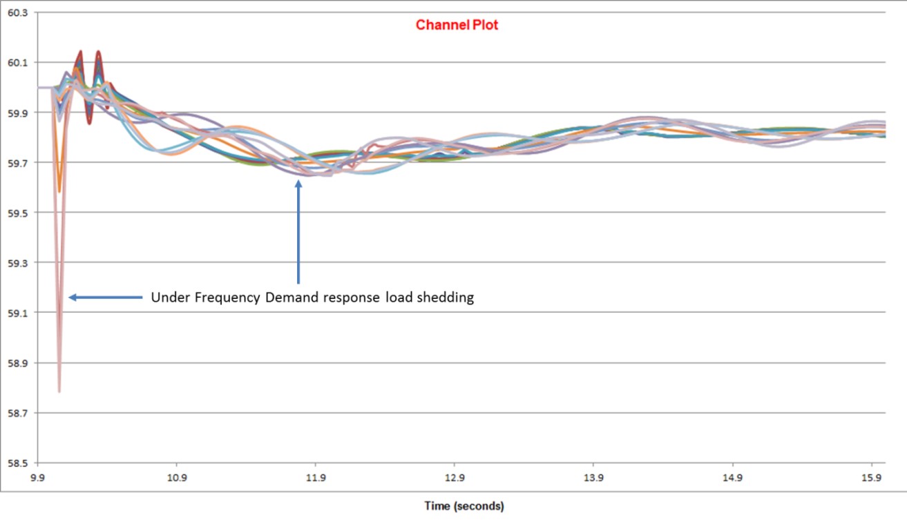
A bus fault that lasted for six cycles was introduced at a large substation. All elements connected to this substation were then tripped to isolate the fault, including a very large power plant. This extreme event did not converge in TransCARE analysis, because the amount of generation loss was higher than the available spinning reserve. Using the DCAT, this extreme event gives a good example of how a non-firm frequency-responsive load shedding scheme acts and sheds a part of the load to restore the balance between generation and load.
A significant amount of generation was lost due to this fault, which was followed by significant underfrequency non-firm load shedding. The fault is introduced at time t = 10 seconds into the dynamic simulation. Graphs of frequency at selected load uses are given in Figure 2.
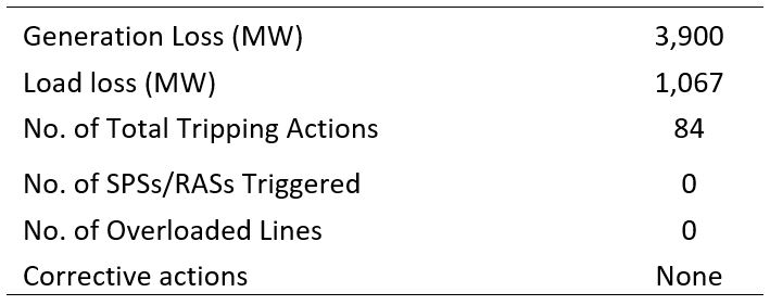
A partial list of the relay tripping sequence observed during the dynamic simulation is given in Table 1. After the dynamic simulation, no control conditions that could trigger SPS/RAS actions were observed. The line overloads observed on the system were below 130% of Rate A and no voltage violations below 0.9 pu were observed. No corrective action was required for this contingency with these protection settings. This contingency resulted in a total of 84 tripping actions with a total generation loss of 3,900 MW and 1,068 MW load loss, as given in Table 2.
Table 1. Partial List of Relay Tripping Sequence for Example 3.
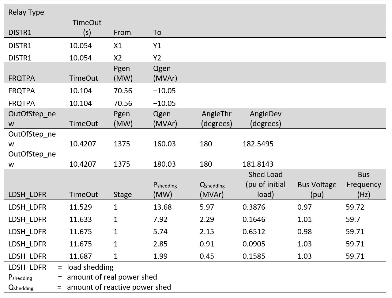
Table 2. Generation and Load Loss Summary for Example 3
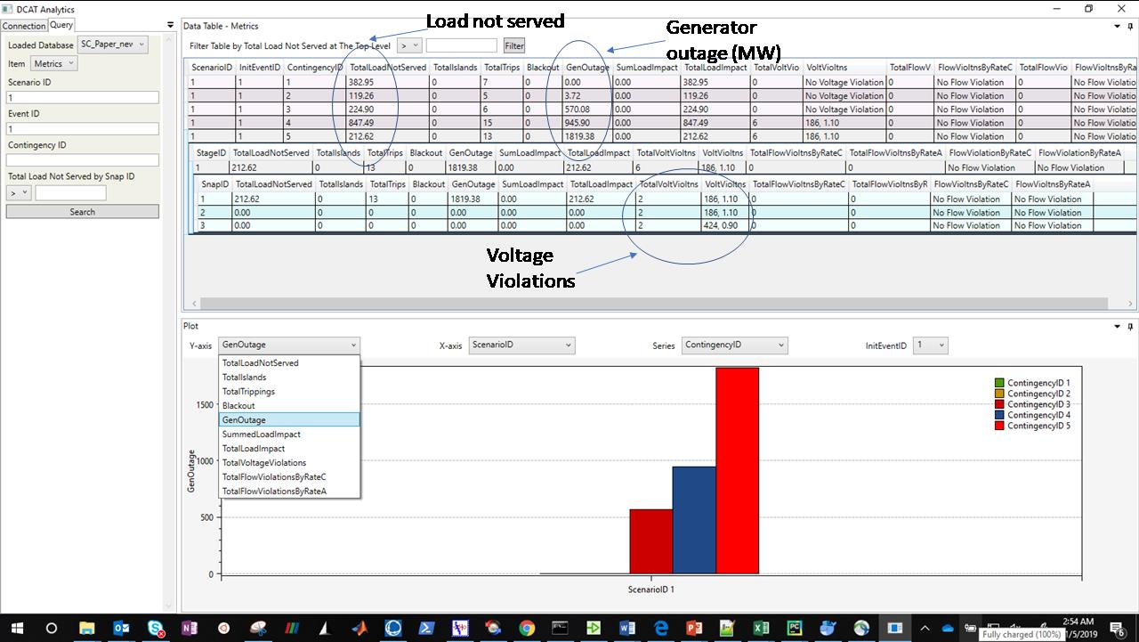
- Database management module for DCAT: Using DCAT’s new automation capability for analyzing various scenarios, all events are simulated, and results are loaded into the database. Using the DCAT GUI, system behavior can be visually explored and analyzed all in one view. The GUI, shown in Fig. 3, has two main parts. The left panel in Fig. 3 is for database connection and query, which are on two separate tabs; the right panel is for visualization of the query results. The figure shows map visualization, including a voltage heat map and overloaded transmission lines. The full-scale interactive data visualization is developed by aggregating data from all contingency scenarios to tell a coherent story with actionable results.
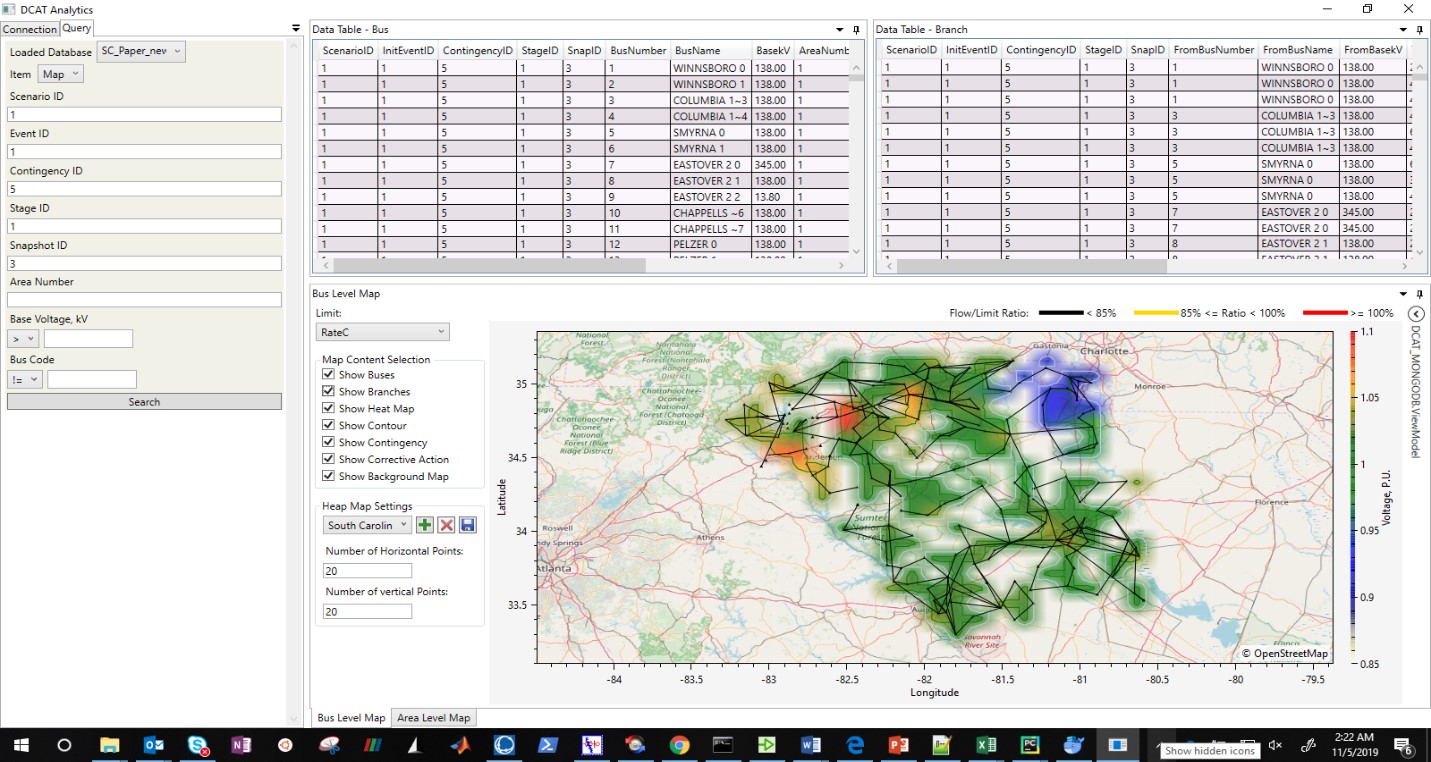
Figure 3. Voltage heat map overloaded transmission lines for an extreme event - DCAT Analytics
The DCAT analytics module is built to rank all simulated contingencies across all events and scenarios, to help the user select where to zoom in for detailed investigation. It can connect directly to data sources and combine, transform, and organize the transformation process into groups or stages (such as voltage violations, flow violations, generation loss, load loss, and RAS actions) using the Query tab.
On the query panel, the user can choose which database to query against. This selection can be changed anytime during the analysis as long as the server connection is established. Each of the query items corresponds to one or more actual queries against the selected database and its collection(s). The returned query results are reorganized for displaying on the right-hand panel of the GUI. Each query item takes some parameters that are field names of the collection(s) in the database; these can be specified by the user. None of these parameters are required but specifying them helps narrow down the queries and shorten the query time. If no parameters are specified, clicking on the “Search” button (at the bottom of the left panel in Fig. 4) returns all records in the collection(s).